Goldbach’s Conjecture and Chebychev’s Bias
During my undergraduate dissertation project looking at the Distribution of Prime Numbers I came across many interesting phenomenomes. Reviewing literature pointed me to two such instances where prime numbers demonstrated there complexity. In investigating these cases I used R to visualise the consequences.
Goldbach’s Conjecture
Goldbach’s Conjecture states that ‘all even real numbers (\(\ge 4\)) can be expressed as a sum of two prime numbers’. The conjecture dates back to the mid-eighteenth century when Christian Goldbach sent a letter to Leonhard Euler to inform him of his discovery.
In almost all cases, there are multiple combinations of prime pairs. Although the conjecture is still widely unsolved it has been shown that the conjecture is true for integers less than \(4 \ \times \ 10^{18}\) using distributed computing.
An interesting property of the conjecture is that there is no apparent pattern in how many combinations of prime pairs exist. The code below shows how seemingly random the frequency of prime pairs are.
library(primes)
library(ggplot2)
library(xtable)
options(xtable.floating = FALSE)
options(xtable.timestamp = "")

# loop parameters
n <- 200
reals <- seq(4, n, by = 2)
prime_factor_pairs <- rep(0, length(reals))
prime_pairs <- rep(0, length(reals))
primes <- generate_primes(max = n)

output <- data.frame(reals = reals,
                     number_of_pairs = prime_factor_pairs,
                     combinations = prime_pairs)

# looping over all reals and checking if the sum of two primes are equal
for (i in 1:length(reals)){
  for (j in 1:length(primes)){
    for (k in 1:length(primes)){
      if (primes[j] + primes[k] == reals[i]){
        if (grepl(primes[j], output$combinations[i])){}
        else{
          output$number_of_pairs[i] <- output$number_of_pairs[i] + 1
          output$combinations[i] <- paste(output$combinations[i],", ", paste("(",primes[j],",",primes[k],")", sep = ""), sep = "")
        }
      }
    }
  }
  output$combinations[i] <- substring(output$combinations[i], 4)
}
output$reals <- as.integer(output$reals)
output$number_of_pairs <- as.integer(output$number_of_pairs)


# Ploting frequency of prime pairs
ggplot2::ggplot(data =output, aes(x = reals, y = number_of_pairs)) +
  geom_col(fill = "tan1") +
  xlab("The even real numbers") +
  ylab("Number of prime pairs") +
  scale_y_continuous(breaks = seq(0, 15, by = 2), limits = c(0, 15)) +
  scale_x_continuous(breaks = seq(0, 200, by = 40), limits = c(0, 200)) +
  ggtitle("Goldbach's Conjecture: Number of prime pairs for each real number up to 200")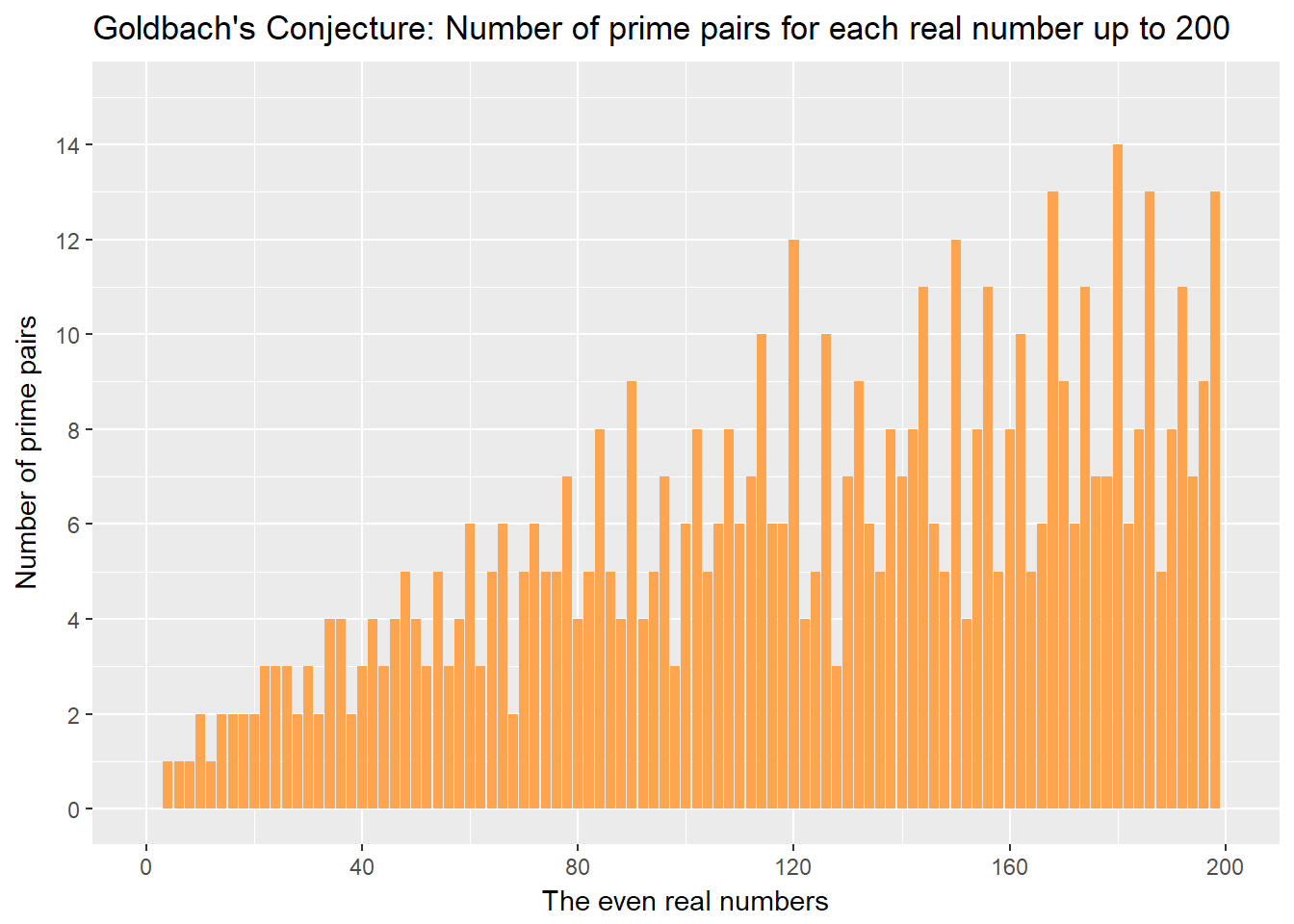
For my dissertation report I also created a table displaying all the combinations of prime pairs for the real numbers up to 100. I used the xtable package to create the LaTeX code that I inserted into the report. Perhaps it would have been easier to do the whole thing in RMarkdown!.
# Creating Latex code for output table
output_table <- xtable::xtable(params$output)
xtable::align(output_table) <- "|l|l|rl|"
xtable::print(output_table, include.rownames = FALSE, tabular.environment = "longtable")
For this blog post I have written the syntax to display the table using RMarkdown and knitr’s kable. The table below shows the prime combinations for the even real numbers, for example \(4\) is made up of \(2 + 2\).
colnames(output) <- c("Reals", "No. of pairs", "Combinations")
knitr::kable(output[1:49,],
             caption = " Prime combinations for real numbers between 4 and 100",
row.names = FALSE)| Reals | No. of pairs | Combinations |
|---|---|---|
| 4 | 1 | (2,2) |
| 6 | 1 | (3,3) |
| 8 | 1 | (3,5) |
| 10 | 2 | (3,7), (5,5) |
| 12 | 1 | (5,7) |
| 14 | 2 | (3,11), (7,7) |
| 16 | 2 | (3,13), (5,11) |
| 18 | 2 | (5,13), (7,11) |
| 20 | 2 | (3,17), (13,7) |
| 22 | 3 | (3,19), (5,17), (11,11) |
| 24 | 3 | (5,19), (7,17), (11,13) |
| 26 | 3 | (3,23), (7,19), (13,13) |
| 28 | 2 | (5,23), (11,17) |
| 30 | 3 | (7,23), (11,19), (13,17) |
| 32 | 2 | (3,29), (13,19) |
| 34 | 4 | (3,31), (5,29), (11,23), (17,17) |
| 36 | 4 | (5,31), (7,29), (13,23), (17,19) |
| 38 | 2 | (7,31), (19,19) |
| 40 | 3 | (3,37), (11,29), (17,23) |
| 42 | 4 | (5,37), (11,31), (13,29), (19,23) |
| 44 | 3 | (3,41), (7,37), (13,31) |
| 46 | 4 | (3,43), (5,41), (17,29), (23,23) |
| 48 | 5 | (5,43), (7,41), (11,37), (17,31), (19,29) |
| 50 | 4 | (3,47), (13,37), (19,31), (43,7) |
| 52 | 3 | (5,47), (11,41), (23,29) |
| 54 | 5 | (7,47), (11,43), (13,41), (17,37), (23,31) |
| 56 | 3 | (3,53), (13,43), (19,37) |
| 58 | 4 | (5,53), (11,47), (17,41), (29,29) |
| 60 | 6 | (7,53), (13,47), (17,43), (19,41), (23,37), (29,31) |
| 62 | 3 | (3,59), (19,43), (31,31) |
| 64 | 5 | (3,61), (5,59), (11,53), (17,47), (23,41) |
| 66 | 6 | (5,61), (7,59), (13,53), (19,47), (23,43), (29,37) |
| 68 | 2 | (7,61), (31,37) |
| 70 | 5 | (3,67), (11,59), (17,53), (23,47), (29,41) |
| 72 | 6 | (5,67), (11,61), (13,59), (19,53), (29,43), (31,41) |
| 74 | 5 | (3,71), (13,61), (31,43), (37,37), (67,7) |
| 76 | 5 | (3,73), (5,71), (17,59), (23,53), (29,47) |
| 78 | 7 | (5,73), (11,67), (17,61), (19,59), (31,47), (37,41), (71,7) |
| 80 | 4 | (7,73), (13,67), (19,61), (37,43) |
| 82 | 5 | (3,79), (11,71), (23,59), (29,53), (41,41) |
| 84 | 8 | (5,79), (11,73), (13,71), (17,67), (23,61), (31,53), (37,47), (41,43) |
| 86 | 5 | (3,83), (7,79), (13,73), (19,67), (43,43) |
| 88 | 4 | (5,83), (17,71), (29,59), (41,47) |
| 90 | 9 | (7,83), (11,79), (17,73), (19,71), (23,67), (29,61), (31,59), (37,53), (43,47) |
| 92 | 4 | (3,89), (13,79), (19,73), (31,61) |
| 94 | 5 | (5,89), (11,83), (23,71), (41,53), (47,47) |
| 96 | 7 | (7,89), (13,83), (17,79), (23,73), (29,67), (37,59), (43,53) |
| 98 | 3 | (19,79), (31,67), (37,61) |
| 100 | 6 | (3,97), (11,89), (17,83), (29,71), (41,59), (47,53) |
Chebychev’s Bias
The definition of a prime number is that it’s only factors are itself and \(1\). Naturally, prime numbers take the form \(4n + 1\) or \(4n + 3\) for \(n \in \mathbb{R}\). For example \(5 \equiv 4n +1,\ n = 1\) and \(11 \equiv 4n +3,\ n = 2\). One interesting property of prime numbers is that the proportion of primes in the form \(4n + 3\) is slightly higher than of form \(4n +1\), as discovered by Chebyshev.
This is not entirely intuitive since the Prime Number Theorem would suggest that approximately half of primes belong to each form, i.e.
\[\begin{equation*} \pi(x; \ 4n + 1) \approx \pi(x; \ 4n + 3) \approx \frac{1}{2} \frac{x}{\ln x}, \end{equation*}\]However, empirical results suggest that this is not the case and primes of the form \(4n + 3\) occur more frequently.
Looking at the first 168 primes plotted, as shown below, this does not suggest a bias towards the \(4n + 3\) form.
library(ggplot2)
plot <- ggplot(data = plot_data) +
  geom_point(aes(x = primes, y = one_mod_four, color = "#F8766D")) +
  geom_point(aes(x = primes, y = three_mod_four, color = "#00BFC4")) +
  scale_color_manual(name = "Type of prime",
                     values = c("#00BFC4" = "#00BFC4", "#F8766D" = "#F8766D"),
                     labels = c("1 mod 4", "3 mod 4")) +
  theme(axis.title.y=element_blank(),
        axis.text.y=element_blank(),
        axis.ticks.y=element_blank(),
        axis.title.x = element_blank()) +
  scale_y_continuous(breaks = c(1), limits = c(0.99, 1.01)) +
  #coord_fixed(ratio = 1) +
  ggtitle("Primes plotted by modulo", paste("First", length(primes), "primes"))
plot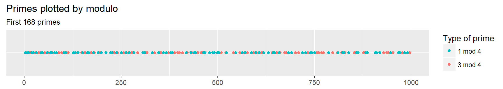
However, looking at the bar chart below we do see a slight bias.
library(ggplot2)
plot2 <- ggplot(data = freq) +
  geom_col(aes(x = label, y = value, fill = label), width = 0.5) +
  guides(fill = "none") +
  xlab("Prime modulo") +
  ylab("Frequency") +
  ggtitle("Primes plotted by modulo - bar chart", paste("First", length(primes), "primes"))
plot2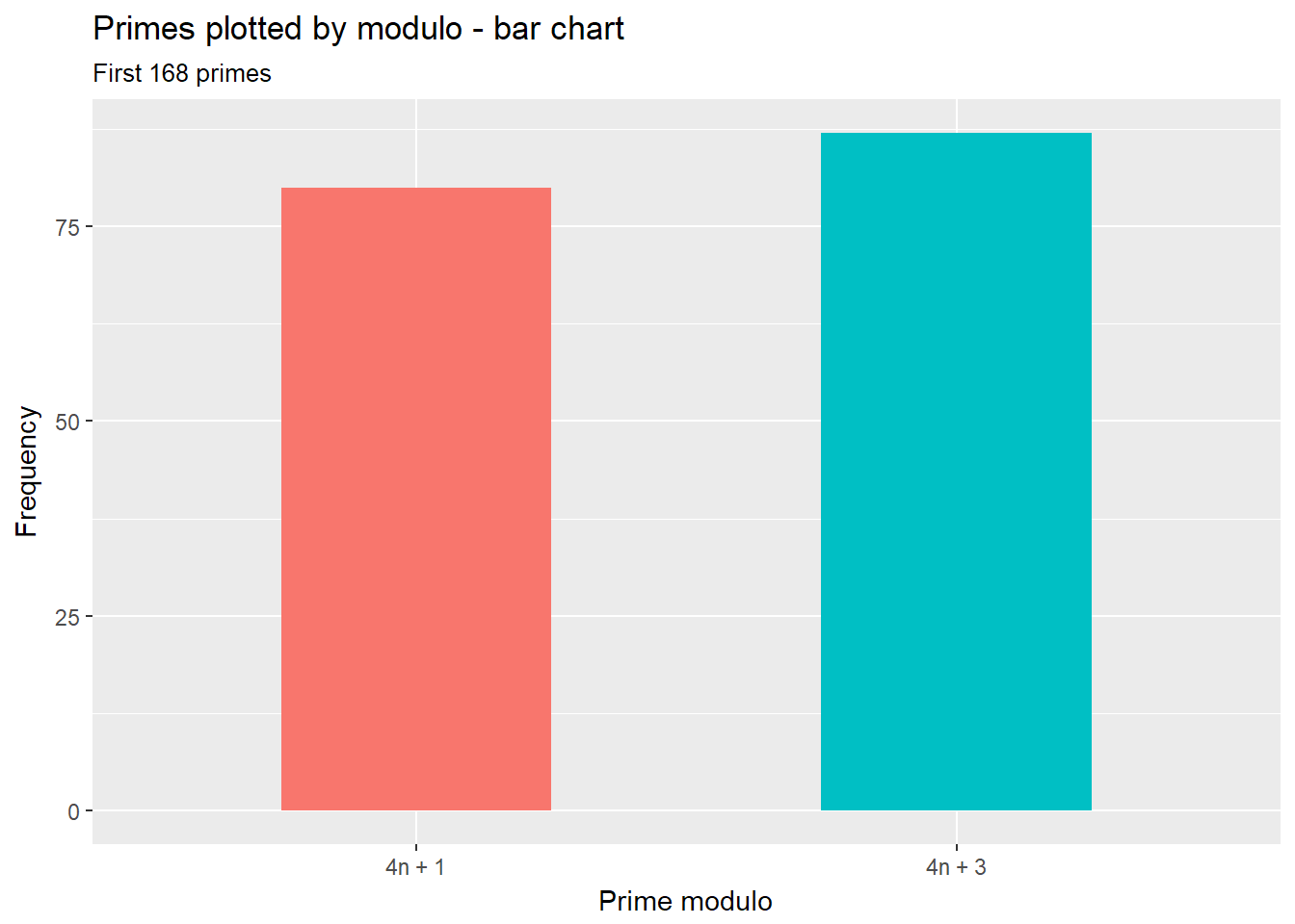
Although the bias does seem to be consistent with a large number of prime numbers, there is in fact a point where the proportion of primes of the form \(4n + 1\) starts to be more common. The bias is true up to the \(26,833^{rd}\) prime number; after this point there is a greater probability of a prime having the form \(4n + 1\).