Prime Counting Functions
Mathematicians have been concerned with counting prime numbers for some time now. In fact the first instance of a so called ‘Prime Counting Function’ comes from the French Mathematician Adrien-Marie Legrendre who in the late eighteenth century conjectured the Prime Number Theory. It stated that one could count the number of primes less that a value \(n\). This was denoted as \(\pi(x)\). For example, for \(x = 10\), \(\pi(10) = 4\) as there are four prime numbers between 0 and 10, these are 2, 3, 5 and 7. An early approximation of the Prime Counting Function was \(\pi(x) \approx \frac{x}{\ln(x)}\).
In this blog post I will explore some of these counting functions using the visualisation package ggplot2 and the primes package that helps generate the list of primes.
# Load the packages we will need
library(primes)
library(ggplot2)
library(reshape, warn.conflicts = FALSE, quietly=TRUE)
library(scales)
We use scales to style the graphs and reshape to make the data easier to work with.
The \(\pi\) counting function
The first counting function we will consider is the \(\pi\) function which, as stated earlier, counts the number of primes less than a given number. This is the function that Mathematicians would like to be able produce. We have to use computers to find the value of this function for higher numbers.
# Set loop paramaters
n <- 5000
x <- seq(1,n, by = 1)
We start by stating the value \(n\) we will evaluate up to and create a vector of ascending numbers from 1 to \(n\).
pi_func <- vector()
for (i in 1:n){
  pi_func[i] <- length(generate_primes(max =i))
}
Next we create pi_func which is a vector of length \(n\). Each position in the vector gives the number of prime numbers less than the position. Using the eariler example, position \(10\) in the vector would show \(4\) as there are \(4\) primes less than \(10\). The generate_primes functions is from the primes package and returns a vector of the primes less than a given number.
dataset <- data.frame(x, pi_func)

pi <- ggplot(data = dataset) +
  geom_line(aes(x = x, y = pi_func)) +
  ylab("Number of primes less than x") +
  ggtitle("The pi counting function")
pi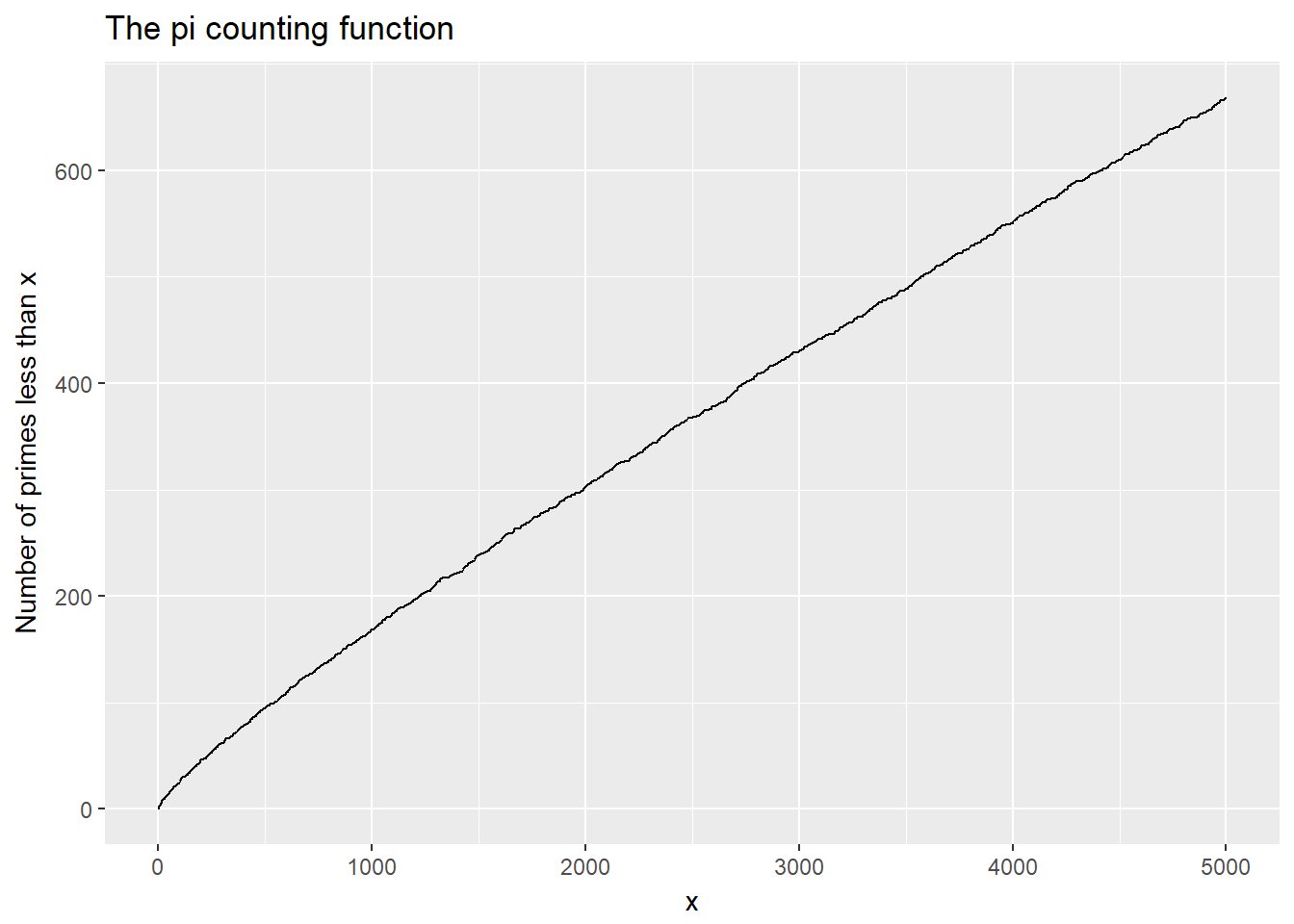
Finally we create a data frame with the sequence of numbers of \(1\) to \(n\) with the number of primes less than that number and create our first graph displaying the \(\pi\) counting function
If we zoom in to the plot we notice that the function exibits a steping motion, which does make sense considering there will be numbers that have the same number of smaller primes. Take for example \(8\), \(9\) and \(10\), all have four primes less.
pi +
  xlim(0, 100) +
  ylim(0, 30)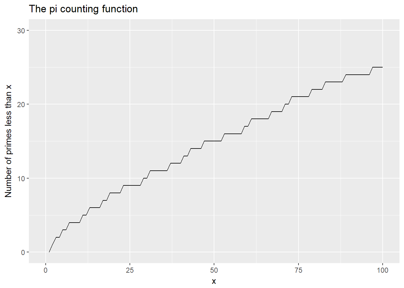
Approximating the \(\pi\) function
Legrendre first approximated the \(\pi\) function to be
\[\pi(x) \approx \frac{x}{ln(x)}\]
approx_func <- x / log(x)
approx_func[c(1,2)] = 0

pi_approx_data <- data.frame(x, pi_func, approx_func)

pi_approx_plot_data <- melt.data.frame(data = pi_approx_data,
                                       id.vars = "x",
                                       measure.vars = c("pi_func", "approx_func"))

ggplot(data = pi_approx_plot_data) +
  geom_line(aes(x = x, y = value, color = variable)) +
  scale_color_discrete(name="Function",
                       breaks=c("pi_func","approx_func"),
                       labels=c("Pi(x)", "x / ln(x)")) +
  ylab("Number of primes less than x") +
  ggtitle("Pi and x / ln(x)")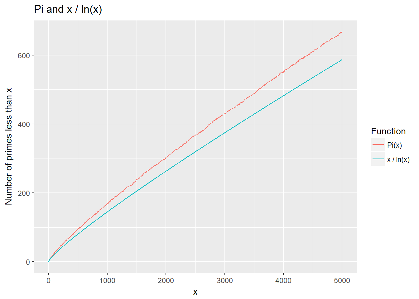
Here we have created a vector of the approximate value of \(\pi\) and manually set the values of \(1\) and \(2\) to be zero. We then gathered the \(\pi\) function and the approximation into a data frame. Next we melted teh data frame using the melt.data.frame from the reshape package which transforms the data so it’s more easily used in ggplot2. Finally we created the graph and set the scale_color_discrete arguments so the legend was nicely formatted.
Gauss’ Li function
German Mathematician Carl Friedrich Gauss had also considered the behaviour of the distribution of primes around 1792/93, even though he was in his teenage years. Similar to Legendre, Gauss studied a list of primes less than \(3,000,000\) which led him to the discovery of the \(Li(x)\) function
\[\begin{equation} Li(x) = \int_{2}^{x}\frac{1}{\ln t}dt. \end{equation}\]The \(Li(x)\) function is more formally known as the Logarithmic Integral Function. Gauss’ estimation for the \(Li(x)\) function was based on the Prime Counting Function \(\pi(x)\)
# Create an empty vector for the Li(x) values
li_values <- vector()

# Create the function inside the integral
li <- function(x){
  1 / log(x)
}

# Integrate from 2 to the n (the length of the vector x)
for (i in 2:length(x)){
  li_values[i] <- as.numeric(substring(as.character(integrate(li, 2, i)), 1, 3)[1])
}
li_values[1] <- 0

# Gather all functions in one data frame
li_func_data <- data.frame(x, pi_func = pi_func, approx_func = approx_func, li_func = li_values)

# Melt the data
li_func_plot_data <- melt.data.frame(li_func_data, id.vars = "x", measure.vars = c("pi_func", "approx_func", "li_func"))
Here we have created the vector of values of the \(Li(x)\) function. Integration is somewhat cumbersome in R so I had to wrap the integrate function a number of times to ensure that I got the correct output.
# Creating the plot
ggplot(data = li_func_plot_data) +
  geom_line(aes(x = x, y = value, color = variable)) +
  ylab("Number of primes for a given x") +
  scale_color_discrete(name="Function",
                       breaks=c("li_func","pi_func","approx_func"),
                       labels=c("Li(x)", "Pi(x)", "x / ln(x)")) +
  ggtitle("Li(x), pi(x) and the pi(x) approximation")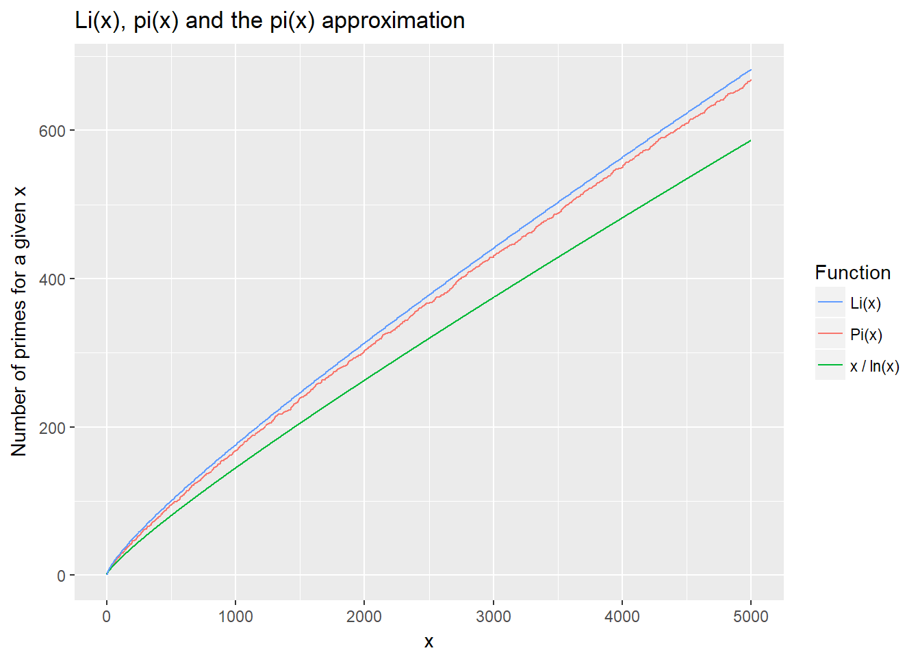
As you can see that Gauss’ \(Li(x)\) function is a much better approximation of \(\pi(x)\) compared to Legrendre’s approximation. \(\frac{x}{ln(x)}\) diverges away very quickly whereas \(Li(x)\) remains a fairly good approximation. However as higher numbers are evaluated both eventually diverge away and cannot be used a good esimation of \(\pi(x)\). Nowadays, Mathematicians interested in the so called Distribution of Primes have turned their attention to the Riemann Hypothesis, which aims to provide a necessary condition for solving Euler’s Product which can in turn be used to generate a list of prime numbers.
Extra: Twin Primes
Not only is there prime counting functions but there are also twin prime counting functions. A pair of twin primes are described to be a prime number that is either 2 less or 2 more than another prime number. For example \(5\) and \(7\), or \(41\) and \(43\) are primes with a difference of 2.
Using the primes package and some simple loops in R we are able to generate a similar \(\pi(x)\) function for twin primes.
# Set loop parameters
y <- seq(1, n)
twin_freq <- vector()

# Carry out loop
for(j in 3:n){
  list_of_primes <- generate_primes(max = j)
  m <- length(list_of_primes)
  prime_diff <- vector()
  prime_diff[1] <- 0
  for (i in 2:m){
    prime_diff[i] <-  list_of_primes[i] - list_of_primes[i - 1]
  }
  twin_primes <- length(which(prime_diff == 2))
  twin_freq[j] <- twin_primes
}

# Gather the data in a data frame
twin_prime_list <- data.frame(y, twin_freq)
twin_prime_list[1, 2] <- 0
twin_prime_list[2, 2] <- 0

# Plot the data
ggplot(data = twin_prime_list) +
  geom_line(aes(x = y, y = twin_freq), color = "blue") +
  ggtitle("Frequence of twin primes for a given pi(x)") +
  xlab("pi(x)") +
  ylab("Frequency of twin primes")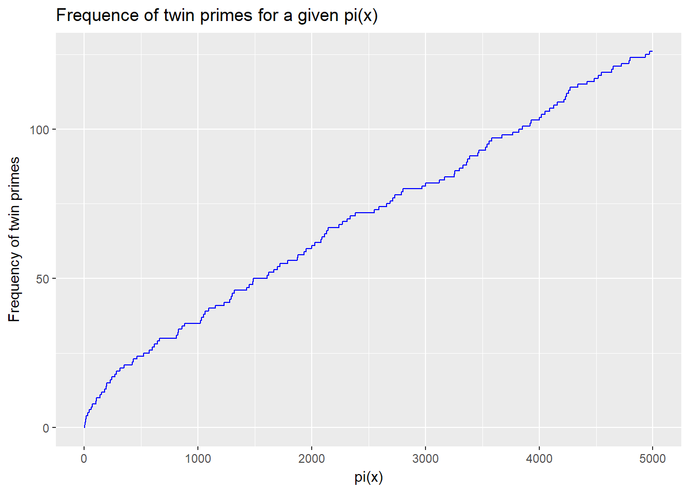
We notice the ’stepping# behaviour again here as we did with the original counting function.
Plotting the twin counting function with the original prime counting function shows something quite interesting:
primes_and_twins <- data.frame(y, pi_func, pi_func_twins = twin_prime_list[, 2])

primes_and_twins_plot_data <- melt.data.frame(data = primes_and_twins,
                                              id.vars = "y",
                                              measure.vars = c("pi_func", "pi_func_twins"))


ggplot(data = primes_and_twins_plot_data) +
  geom_line(aes(x = y, y = value, color = variable)) +
  scale_color_discrete(name="Type of prime",
                       breaks=c("pi_func","pi_func_twins"),
                       labels=c("Normal prime", "Twin prime")) +
  ggtitle("Prime and Twin Primes") +
  ylab("Number of primes")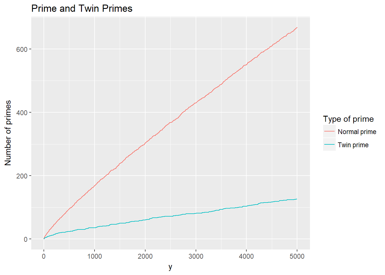
The instances of twin primes are of course far less than that of normal primes but what is interesting is that the number of twin primes is very steadily increasing, much like that of normal primes. The so called twin prime conjecture is not yet proven but it is assumed that there are an infinite number of twin primes.