Are My Friends Negative Tweeters? (Part 2)

This is part 2 of a project I worked on to determine if my friends are negative tweeters. In this part I retrieve my friend’s tweets and run our model against it to determine the sentiment of the tweets.

Haven’t seen part 1? Click here

Accessing my friend’s timelines

To access my friend’s tweets I had to create an application on Twitter Apps and input my keys and tokens into the setup_twitter_oauth function from the twitteR package. This enabled me to connect with the Twitter API and retrieve tweets.

setup_twitter_oauth(consumer_key = ..., 
                    consumer_secret = ..., 
                    access_token= ..., 
                    access_secret= ...)

For ease I created a vector for the column names and my friend’s twitter handles.

# Select relevant variables
columns <- c("text",
             "created",
             "screenName")

# usernames of my friends
users <- c("friend 1",
           "friend 2",
           ...)

Once I had the list of twitter handles I created a function that takes a user’s handle, accesses the Twitter API and returns the user’s tweets. I then used this function on the vector of friend’s twitter handles.

# custom function to retrieve my friends timelines
get_tweets <- function(x){
  user_timeline_listed <- userTimeline(x, n = 1000)
  user_timeline <- do.call("rbind", lapply(user_timeline_listed, as.data.frame))[columns]
  return(user_timeline)
}

# Applying the custom function to the vector of usernames
tweets <- do.call("rbind", lapply(lapply(users, get_tweets), as.data.frame))

I then decided to clean the Tweets myself a little to help with the Natural Language Processing later.

# Clean up tweets
tweets_cleaned <- tweets
tweets_cleaned$text<- sapply(tweets_cleaned$text, function(row) iconv(row, "latin1", "ASCII", sub=""))
tweets_cleaned$text <- gsub("@\\w+ *", "", tweets_cleaned$text)
tweets_cleaned$text <- gsub("#\\w+ *", "", tweets_cleaned$text)
tweets_cleaned$text <- gsub(" ?(f|ht)(tp)(s?)(://)(.*)[.|/](.*)", "", tweets_cleaned$text)

I then did four things:

change the column names to be consistent with the Kaggle_tweets dataset
add two columns; an empty column of Sentiment (to be updated after using the model) and the Friends column that will be used to differentiate my friend’s tweets
reorder the column orders to be consistent with the other dataset
change the date format to match the other dataset

colnames(tweets_cleaned) <- c("Tweet", "Date", "User")

tweets_cleaned$Sentiment <- NA
tweets_cleaned$Friends <- 1

tweets <- tweets_cleaned %>% 
  select(Sentiment, Date, User, Tweet, Friends) %>% 
  filter(Tweet != "")

tweets$Date <- as_date(tweets$Date, tz = NULL)

Creating another corpus

In part 1 of this project I created a random forest classifier using the Kaggle dataset to verify the accuracy. To determine the sentiment of my friend’s tweets I will use all of that data to train a new model and unleash it upon my friend’s tweets.

Step one was to merge the data using a helpful function from dplyr. I also added a Friends column to the kaggle dataset.

kaggle_tweets$Friends <- 0

model_data <- bind_rows(kaggle_tweets, tweets)

The next step was to create the corpus, process the tweets and output a sparse matrix as I did in part 1.

new_corpus = VCorpus(VectorSource(model_data$Tweet))          # Creating the corpus
new_corpus = tm_map(new_corpus, content_transformer(tolower)) # all letters to lowercase
new_corpus = tm_map(new_corpus, removeNumbers)                # removing numbers
new_corpus = tm_map(new_corpus, removePunctuation)            # removing punctuation
new_corpus = tm_map(new_corpus, removeWords, stopwords())     # removing stopwords
new_corpus = tm_map(new_corpus, stemDocument)                 # steming words
new_corpus = tm_map(new_corpus, stripWhitespace)              # removing whitepace

dtm <- DocumentTermMatrix(new_corpus)                         # Transforming corpus to a workable matrix
dtm_sparse <- removeSparseTerms(dtm, 0.99996)
friends_dataset <- as.data.frame(as.matrix(dtm_sparse))       # transforming into a data frame

I then added the Sentiment to the tweets. At this stage on the kaggle tweets (signified by Friends = 0) had a given sentiment and my friend’s tweets (Friends = 1) had no sentiment.

friends_dataset$Sentiment <- model_data$Sentiment
friends_dataset$Friends <- model_data$Friends

friends_dataset <- friends_dataset %>% 
  select(Sentiment, Friends, everything())

Finally I split the data into a training set (kaggle tweets) and a results set (friend’s tweets) and created the classifier.

# Split into training and results sets
new_train_set <- filter(friends_dataset, Friends == 0)
new_results_set <- filter(friends_dataset, Friends == 1)

# Train the model
classifier <- randomForest(x = new_train_set[-c(1, 2)],
                           y = new_train_set$Sentiment,
                           ntree = 5)

Results

Once I had the classifier all I had to do was update the sentiment of my friend’s tweets.

tweets$Sentiment <- predict(classifier, newdata = new_results_set[-c(1,2)])

Now for the exciting part; visualising the results.

Overall Sentiment of tweets

tweets_sentiment <- select(tweets, Sentiment) %>% 
  group_by(Sentiment) %>% 
  summarise(Sum = n()) %>% 
  ggplot() +
  geom_bar(aes(x = "", y = Sum, fill = Sentiment), stat = "identity", width = 1) +
  coord_polar(theta = "y" ) +
  theme(axis.text = element_blank(),
        axis.ticks = element_blank(),
        panel.grid  = element_blank(),
        axis.title = element_blank(),
        axis.line = element_blank(),
        legend.position = "bottom",
        legend.title = element_blank(),
        plot.title = element_text(hjust = 0.5),
        plot.subtitle = element_text(hjust = 0.5, face = "italic", size = 12)) +
  ggtitle("Sentiment of Friend's Tweets",
          paste("Accessed", Sys.Date(), "via TweetR package"))

# Kaggle sentiment
kaggle_tweets_sentiment <- select(kaggle_tweets, Sentiment) %>% 
  group_by(Sentiment) %>% 
  summarise(Sum = n()) %>% 
  ggplot() +
  geom_bar(aes(x = "", y = Sum, fill = Sentiment), stat = "identity", width = 1) +
  coord_polar(theta = "y" ) +
  theme(axis.text = element_blank(),
        axis.ticks = element_blank(),
        panel.grid  = element_blank(),
        axis.title = element_blank(),
        axis.line = element_blank(),
        legend.position = "bottom",
        legend.title = element_blank(),
        plot.title = element_text(hjust = 0.5),
        plot.subtitle = element_text(hjust = 0.5, face = "italic", size = 12)) +
  ggtitle("Sentiment of Kaggle Tweets",
          "Random sample of 10,000 tweets")

# Plot side by side
sentiment_plot <- plot_grid(tweets_sentiment, kaggle_tweets_sentiment, ncol = 2)
sentiment_plot

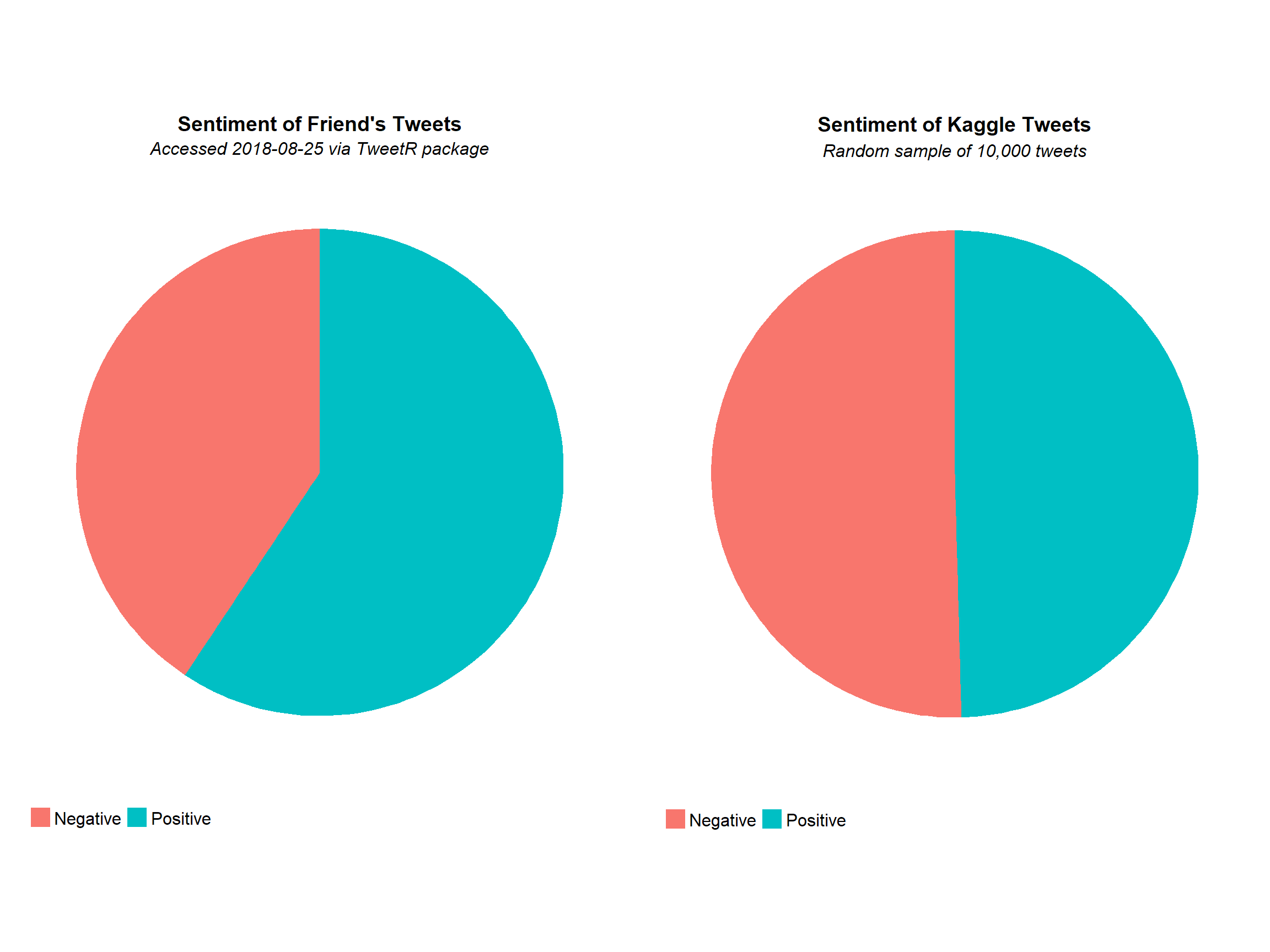
It seems that my hypothesis was not correct and that, in general, my friends tend to be more positive in their tweets compared to the average. Perhaps it is my outlook on the tweets that is more negative than positive. Anyway, it was interesting to see the overall sentiment of the kaggle tweets with them being almost equally likely negative as positive.

Friend’s Sentiment

tweets_sentiment_by_user <- ggplot(data = tweets) +
  geom_bar(aes(x = Sentiment, fill = Sentiment)) + 
  facet_wrap(~ User) +
  ylab("Number of Tweets") +
  theme(legend.position = "bottom",
        legend.title = element_blank(),
        axis.text.x = element_blank(),
        axis.ticks.x = element_blank(),
        strip.text.x = element_text(size = 10),
        axis.text.y = element_text(size = 9),
        plot.title = element_text(hjust = 0),
        plot.subtitle = element_text(face = "italic")) +
  ggtitle("Sentiment of friend's tweets by individual friend",
          paste("Accessed", Sys.Date(), "via TweetR package; retrieved last 1000 tweets of each friend"))
tweets_sentiment_by_user

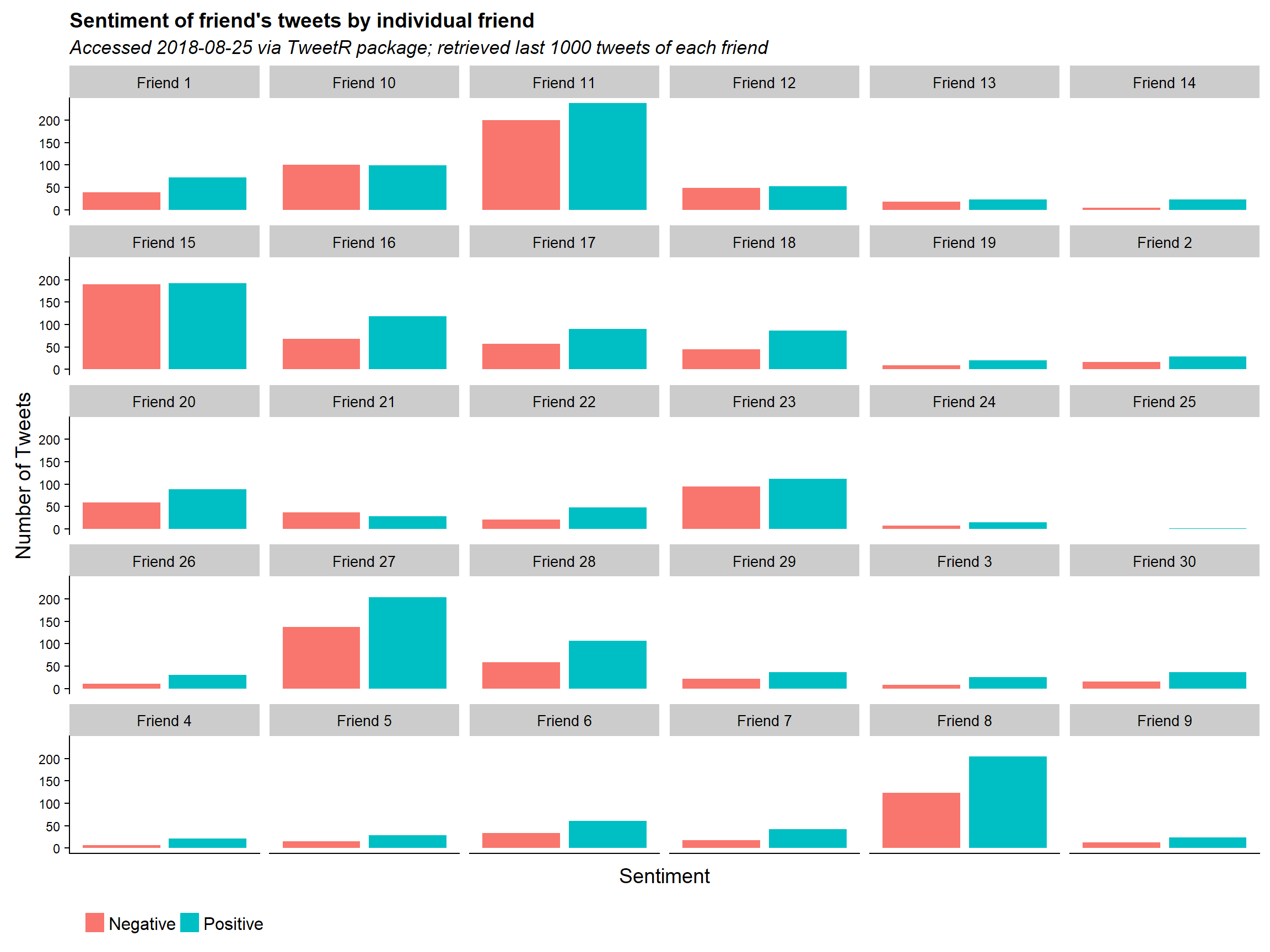
It is quite clear that some of my friends are more active tweeters than others. In general however the trend from the first graph can be seen among most of my friends. There are a few exceptions; friend 15 for example tends to be slightly more negative than positive.

You may notice that there are fewer than 1,000 tweets for each friend. This is an issue I found while using the user_timeline_listed function. I couldn’t figure out why but when asking to retrieve 1,000 tweets I would only get about a third of this for each friend. Additionally some of my friends had far less than 1,000 tweets.

Sentiment by Weekday

# Create a weekday factor variable
tweets$Weekday <- factor(weekdays.Date(tweets$Date, abbreviate = FALSE),
                         levels= c("Monday", "Tuesday", "Wednesday", 
                                   "Thursday", "Friday", "Saturday", "Sunday"),
                         labels = c("Mon", "Tue", "Wed", "Thu", "Fri", "Sat", "Sun"))
kaggle_tweets$Weekday <- factor(weekdays.Date(kaggle_tweets$Date, abbreviate = FALSE),
                                levels= c("Monday", "Tuesday", "Wednesday", 
                                          "Thursday", "Friday", "Saturday", "Sunday"),
                                labels = c("Mon", "Tue", "Wed", "Thu", "Fri", "Sat", "Sun"))

# Friend's sentiment by weekday
tweets_sentiment_by_weekday <- ggplot(data = tweets) +
  geom_bar(aes(x = Sentiment, fill = Sentiment)) +
  facet_grid(. ~ Weekday) +
  theme(legend.position = "bottom",
        legend.title = element_blank(),
        axis.text.x = element_blank(),
        axis.ticks.x = element_blank()) +
  ylab("Number of Tweets") +
  ggtitle("Friend's Sentiment by Weekday")

# Kaggle sentiment by weekday
kaggle_tweets_sentiment_by_weekday <- ggplot(data = kaggle_tweets) +
  geom_bar(aes(x = Sentiment, fill = Sentiment)) +
  facet_grid(. ~ Weekday) +
  theme(legend.position = "bottom",
        legend.title = element_blank(),
        axis.text.x = element_blank(),
        axis.ticks.x = element_blank()) +
  ylab("Number of Tweets") +
  ggtitle("Kaggle tweets Sentiment by Weekday")

# Plot side by side
weekday_sentiment_plot <- plot_grid(tweets_sentiment_by_weekday, kaggle_tweets_sentiment_by_weekday, ncol = 2)
weekday_sentiment_plot

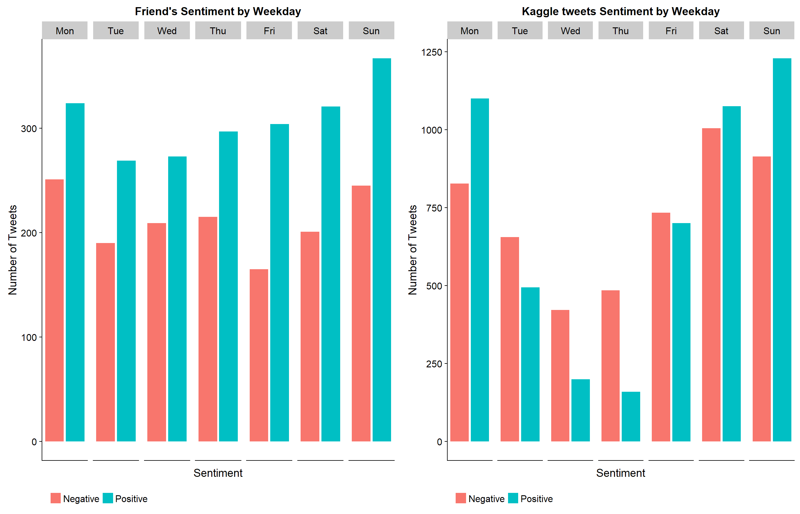
The sentiment trend of my friends continues when split by the weekday a tweet is sent. A tweet is more likely to be positive than negative regardless of the day of the week. What surprised me the most was the trends seen in the kaggle tweets; tweets are more likely to be negative on a Thursday and Wednesday and almost equally likely on Friday and Saturday. I would have thought people would be more positive towards the end of the week.

Tweets by Weekday

# Friend's tweets by weekday
tweets_by_weekday <- ggplot(data = tweets) +
  geom_bar(aes(x = Weekday, fill = Weekday)) +
  coord_flip() +
  theme(legend.position = "none") +
  ggtitle("Tweets by weekday") +
  ylab("Number of tweets")

# Kaggle tweets by weekday
kaggle_tweets_by_weekday <- ggplot(data = kaggle_tweets) +
  geom_bar(aes(x = Weekday, fill = Weekday)) +
  coord_flip() +
  theme(legend.position = "none") +
  ggtitle("Kaggle tweets by weekday") +
  ylab("Number of tweets")

# Plot side by side
weekday_plot <- plot_grid(tweets_by_weekday, kaggle_tweets_by_weekday, ncol = 2)
weekday_plot

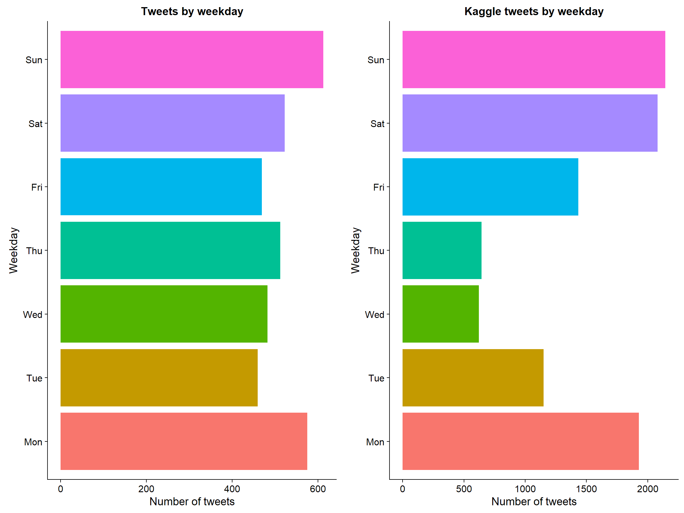
Just out of interest I wanted to see which days were more popular for tweeting. It appears that Mondays and Sundays are the most popular and tweets tend to die down midweek. This is more apparent in the kaggle tweets compared to my friends.

I would have liked to split the tweets by hour or even import some location data (if this is possible) as this could have added another layer of interest. Perhaps I will return to this type of project in the future.

Overall this was a very interesting project. I find it a lot easier to retain interest when dealing with data I can relate to. Scraping my friend’s tweets felt somewhat naughty considering none of them will ever have known I had done so (unless they ever get around to reading my blog posts…) but hey, that’s public data for you.