Getting data

Having to watch all 20 MCU movies and noting the time each character appears on screen would have really discouraged me from completing this project. Fortunately the nice people at the IMDb have done precisely this and published the list of character screen time for each movie. This was a relief for me. There was still the issue that I would need to copy all the data in a way in which It could be analysed in R.

I could have manually entered the data into an empty data frame but that didn’t seem clever or flashy enough for a Data Science blog post. Instead I decided to scrape the data using the R package rvest which provides a number of really useful functions for web scraping.

I also used a number of packages to help with the analysis:

• dplyr, lubridate and tidyr were used to help with data wrangling and manipulation

• reshape2 was used to transform the web data to a more manageable data frame

• The rapportools package provided a helpful function to check if cells were blank

• ggplot2 was used to make the visualisations

# Packages
library(rvest)
library(lubridate)
library(dplyr)
library(ggplot2)
library(reshape2)
library(tidyr)
library(rapportools)

To get the data from the IMDb website I had to open a connection and read all the HTML elements of the website. This was done using rvest’s read_html function.

# Get website URL
url <- "https://www.imdb.com/list/ls066620113/?sort=list_order,asc&st_dt=&mode=detail&page=1"

# Read url html
webpage <- read_html(url)

I then wanted to collect some information about the films, including;

• Title of the film

• Year of release

• Order in franchise

• Character screen time in minutes

To do this I had to select the HTML element that I wanted to read into R. The html_nodes function scrapes the required HTML element. In the first case I scraped the order of release which corresponded with the ‘.text-primary’ element. I located the element using an extension for Chrome called Selector Gadget.

I then converted the HTML element into text using the html_text function.

# Rank - order of releases

# Using CSS selectors to scrape the rankings section
rank_data_html <- html_nodes(webpage,'.text-primary')

# Convert 
rank_data <- html_text(rank_data_html)
rank_data <- as.numeric(rank_data)

I then repeated this process for the year of release and title. I created a data frame of the rank (order of release) with the title to be used later. For the year of release I had to remove the first three elements since I couldn’t get the specific HTML element using Selector Gadget. I also had to take a sub-string so that the date was in the correct format. As with the title I created a data frame of rank and date to be used later.

# Title

# Using CSS selectors to scrape the rankings section
title_data_html <- html_nodes(webpage,'.lister-item-header a')

# Convert 
title_data <- html_text(title_data_html)
title_data <- data.frame(rank = rank_data, title = title_data)



# Year

# Using CSS selectors to scrape the rankings section
date_data_html <- html_nodes(webpage,'.text-muted.unbold')

# Convert 
date_data <- html_text(date_data_html)
date_data <- date_data[-c(1:3)]
date_data <- substr(date_data, 2, 5)
date_data <- data.frame("rank" = rank_data, "date" = date_data)

The final HTML element I needed was the character screen times which was by far the most difficult to retrieve.

# Screen Time

screentime_data_html <- html_nodes(webpage, ".mode-detail .list-description p")

# Convert
screentime_data <- html_text(screentime_data_html)

When converting the HTML element to text the screen times were converted as a single string for each movie. Additionally, the character screen time was joined in the same string as the character name. For example, the element for Iron Man looked like this:

head(screentime_data, 1)

## [1] "Tony Stark / Iron Man <77:15>\nPepper Potts <23:15>\nObadiah Stane / Iron Monger <22>\nProfessor Ho Yinsen <10:45>\nLt. Col. James \"Rhodey\" Rhodes <8:15>\nRaza <6>\nAgent Phil Coulson <3:45>\nChristine Everhart <3:45>\nAbu Bakaar <1:45>\nHarold \"Happy\" Hogan <1:15>\nDirector Nick Fury <:15>\nJ.A.R.V.I.S. <v>"

To get around this I split the strings using the strsplit function which created individual strings for each character. I then melted the data so that each row would give the character and screen time string.

screentime_data <- strsplit(screentime_data, split = "[\n]")
screentime_data <- melt(screentime_data)
head(screentime_data, 10)

##                                    value L1
## 1          Tony Stark / Iron Man <77:15>  1
## 2                   Pepper Potts <23:15>  1
## 3       Obadiah Stane / Iron Monger <22>  1
## 4            Professor Ho Yinsen <10:45>  1
## 5  Lt. Col. James "Rhodey" Rhodes <8:15>  1
## 6                               Raza <6>  1
## 7              Agent Phil Coulson <3:45>  1
## 8              Christine Everhart <3:45>  1
## 9                      Abu Bakaar <1:45>  1
## 10           Harold "Happy" Hogan <1:15>  1

Cleaning the data

Once I had all the necessary data I had to do a few things to make it more manageable. The first of which was to create a dataset containing everything we needed. I then reordered the data and changed the variable names.

# Add title and date to the dataset
screentime_data$title <- title_data$title[match(screentime_data$L1, table = title_data$rank)]

screentime_data$date <- date_data$date[match(screentime_data$L1, table = date_data$rank)]

# Reorder and rename
screentime_data <- select(screentime_data, L1, title, date, value)                                             
colnames(screentime_data) <- c("Rank",
                               "Title",
                               "Date",
                               "Character")

I then had to deal with the character/screen time string. Using tidyr’s separate function I was able to split the variable into two; the character and the screen time. I also removed the brackets around the screen time.

# Separate the character/screentime variable to two separate variables 
screentime_data <- separate(screentime_data, 
         col = Character, 
         into = c("Character", "Screentime"), 
         sep = "<", 
         remove = TRUE, 
         convert = FALSE)

# Clean the screentime variable
screentime_data$Screentime <- gsub(">", "", screentime_data$Screentime)

head(screentime_data)

##   Rank    Title Date                       Character Screentime
## 1    1 Iron Man 2008          Tony Stark / Iron Man       77:15
## 2    1 Iron Man 2008                   Pepper Potts       23:15
## 3    1 Iron Man 2008    Obadiah Stane / Iron Monger          22
## 4    1 Iron Man 2008            Professor Ho Yinsen       10:45
## 5    1 Iron Man 2008 Lt. Col. James "Rhodey" Rhodes        8:15
## 6    1 Iron Man 2008                           Raza           6

Next I separated the screen time into minutes and seconds using the separate function again.

# Separate the minute/second variable to two separate variables 
screentime_data <- separate(screentime_data, 
                            col = Screentime, 
                            into = c("Minutes", "Seconds"), 
                            sep = ":", 
                            remove = TRUE, 
                            convert = FALSE)

When splitting the screen time into minutes and seconds I realised that this caused a few problems. Firstly, if a character had less than a minute in a film, much like Thanos in his many post-credit cameos, then the minute variable would be blank. Secondly, some characters, like J.A.R.V.I.S (who is not actually seen on screen), were noted down as \(<V>\).

To deal with the first problem I created a custom function that checked if a cell was empty or not and enter ‘0’ if it was. rapportools’s is.blank function was used to check blank cells. I then applied this to the Minutes variable. After, I converted the Minutes variable into a numeric type which had the added benefit of turning character strings into NAs. I could then filter out NAs and remove characters with no formal screen time.

# Custom function to turn blanks into "0"
check_blanks <- function(x){
  blank <- is.empty(x)
  if(blank == TRUE)
    return(0)
  else 
    return(x)}

# Applying function to Minutes
screentime_data$Minutes <- sapply(screentime_data$Minutes, check_blanks)

# Coerce Minutes into numeric
screentime_data$Minutes <- as.numeric(screentime_data$Minutes)

# Filter out characters with no screentime
screentime_data <- filter(screentime_data,
                          !is.na(Minutes))

I was also able to filter out the NAs in the Seconds column which resulted from having no seconds.

# Change Second NAs to "0"
screentime_data$Seconds[is.na(screentime_data$Seconds)] <- 0

# Numeric numbers
screentime_data$Seconds <- as.numeric(screentime_data$Seconds)

Finally I could created a combined Time variable that could be understood by ggplot2. I also trimed the whitespace on the Character variable.

# Create a combined minute/second variable
screentime_data <- mutate(screentime_data, Time = Minutes + (Seconds / 60))

# Trim whitespace
screentime_data$Character <-trimws(screentime_data$Character)

Results

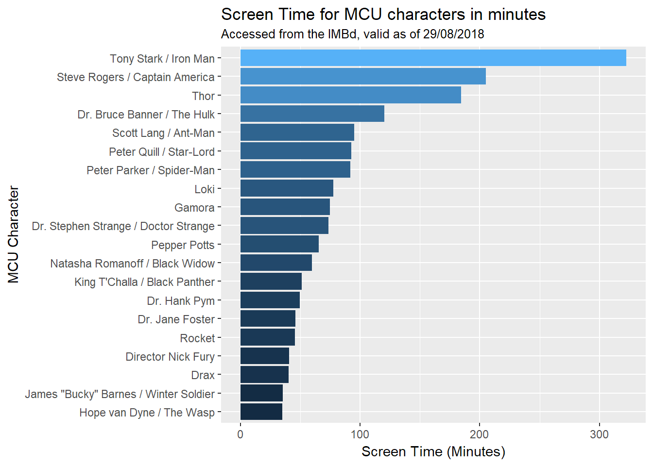
Now that I had a clean dataset I wanted to explore it. I first looked at the top 20 characters in terms of screen time:

actor_screentime <- screentime_data %>% 
  group_by(Character) %>% 
  summarise("Screen_Time" = sum(Time)) %>% 
  top_n(20) %>% 
  ungroup() %>% 
  arrange(Screen_Time) %>% 
  ggplot(aes(x = reorder(Character, Screen_Time), y = Screen_Time, fill = log(Screen_Time))) +
  geom_col() +
  coord_flip() +
  ggtitle("Screen Time for MCU characters in minutes",
          "Accessed from the IMBd, valid as of 29/08/2018") +
  xlab("MCU Character") +
  ylab("Screen Time (Minutes)") +
  theme(legend.position = "none")
actor_screentime

No surprise that Iron Man, Captain America and Thor dominate the screens with them being flagship characters in the comics and movies. I was, however, surprised that Ant-Man was ranked so high, but then he has had more solo movies than Black Panther who seems to be a more integral part of the MCU. No surprise to see the Guardians of the Galaxy taking spots in the top twenty.

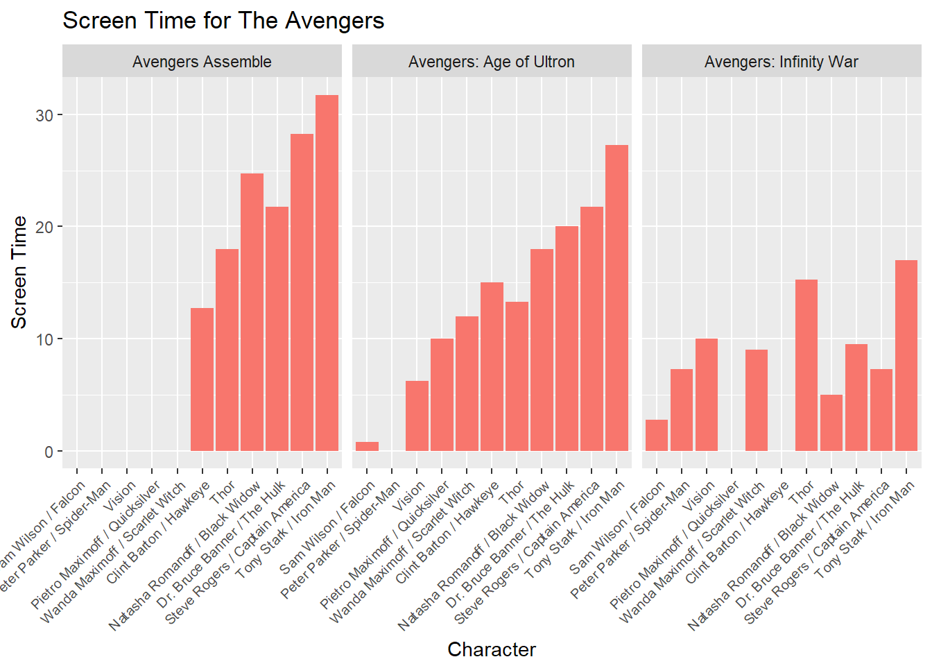
I was also interested to see which of the mainstay Avengers had the most screen time and how this evolved over the course of the three Avenger titles. To do this I had to subset the dataset by the Title and Character variables to keep only the main Avengers and their screen times in the three Avengers movies. I had to manually change the names of some of the characters since they changed from movie to movie which was a little annoying.

avengers <- c("Tony Stark / Iron Man",
              "Steve Rogers / Captain America",
              "Agent Natasha Romanoff / Black Widow",
              "Dr. Bruce Banner / The Hulk",
              "Thor",
              "Agent Clint Barton / Hawkeye",
              "Clint Barton / Hawkeye",
              "Wanda Maximoff / Scarlet Witch",
              "Pietro Maximoff / Quicksilver",
              "Vision",
              "Col. James 'Rhodey' Rhodes / War Machine",
              "Sam Wilson / Falcon",
              "Peter Parker / Spider-Man",
              "Steve Rogers",
              "James 'Bucky' Barnes / White Wolf",
              "Natasha Romanoff / Black Widow")

Avengers_movies <- screentime_data %>% 
  filter(Title %in% c("Avengers Assemble", "Avengers: Age of Ultron", "Avengers: Infinity War"),
         Character %in% avengers)
Avengers_movies$Character[3] <- "Natasha Romanoff / Black Widow"
Avengers_movies$Character[6] <- "Clint Barton / Hawkeye"
Avengers_movies$Character[23] <- "Steve Rogers / Captain America"

Avengers_movies_plot <- ggplot(data = Avengers_movies) +
  geom_col(aes(x = reorder(Character, Time), y = Time), fill = "#F8766D") +
  facet_grid(. ~ Title) +
  theme(axis.text.x = element_text(angle = 45, hjust = 1, size = 7.5),
        legend.position = "none") +
  ggtitle("Screen Time for The Avengers") +
  xlab("Character") +
  ylab("Screen Time")
Avengers_movies_plot  

Again, no surprise that Iron Man dominates throughout the three movies. It is interesting that Captain America had far less screen time in ‘Infinity War’ but is reflective of the criticism the film received saying that the character had too little a role. We do also see that by the third movie the screen time is much more even which makes sense considering the branching narrative the film portrays.

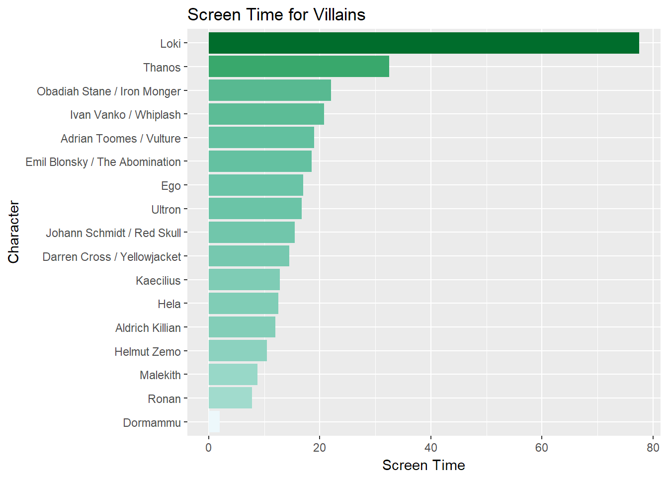
They say that a hero is nothing without their villain, and the MCU has offered up some memorable villains over the last 10 years. I was interested to see which of the main villains received the most screen time.

Villains <- c("Ivan Vanko / Whiplash",
              "Emil Blonsky / The Abomination",
              "Malekith",
              "Dormammu",
              "Ronan",
              "Kaecilius",
              "Darren Cross / Yellowjacket",
              "General Ross",
              "Hela",
              "Aldrich Killian",
              "Helmut Zemo",
              "Ultron",
              "Obadiah Stane / Iron Monger",
              "Thanos",
              "Johann Schmidt / Red Skull",
              "Ego",
              "Adrian Toomes / Vulture",
              "N'Jadaka / Erik 'Killmonger' Steven",
              "Loki")

Villains_plot <- screentime_data %>% 
  filter(Character %in% Villains) %>% 
  group_by(Character) %>% 
  summarise(Time = sum(Time)) %>% ggplot() +
  geom_col(aes(x = reorder(Character, Time), y = Time, fill = -log(Time))) +
  scale_fill_distiller(palette = "BuGn") +
  coord_flip() +
  theme(legend.position = "none") +
  ggtitle("Screen Time for Villains") +
  xlab("Character") +
  ylab("Screen Time")
Villains_plot

No surprise at all that Loki dominates the screen for the Villains with his 5 appearances in the MCU so far, though only once as the main antagonist. The second most featured Villain is Thanos although four of his appearances are cameos or minor roles. It’s not until ‘Infinity War’ in which he rakes up the most screen time with 31 minutes, more than any Villain or hero in that movie.

With the MCU about to enter it’s fourth phase I am sure that the old characters will begin to fade off our screens to make room for new blood. I would certainly be interested to see how these visualisations would look after another 10 years of Marvel.